Processing software: iMOSFLM(integration) Aimless(scaling)
STARANISO version: 3.0.17 (1-Oct-2025) Run on: Thu, 04 Dec 2025 03:54:34 +0100.
Using MTZ column labels: IMEAN SIGIMEAN I(+) SIGI(+) I(-) SIGI(-)
Unit cell and space group: 49.800 84.370 108.000 90.00 90.00 90.00 'P 21 21 21'
Nominal diffraction range: 66.487 2.000
Input reflection count: 31486
Unique reflection count: 31254
Diffraction cut-off criterion: Local <I/sd(I)> = 1.20
Semi-axis d-spacings (Ang.) and corresponding principal axes of the ellipsoid fitted to the
diffraction cut-off surface:
Diffraction limit #1: 1.995 ( 1.0000, 0.0000, 0.0000) a*
Diffraction limit #2: 1.887 ( 0.0000, 1.0000, 0.0000) b*
Diffraction limit #3: 1.930 ( 0.0000, 0.0000, 1.0000) c*
The principal axes are given as direction cosines relative to the orthonormal basis (standard PDB
convention), and also in terms of reciprocal unit-cell vectors.
Worst diffraction limit after cut-off:
2.195 at reflection 22 1 12 in direction 0.877 a* + 0.040 b* + 0.478 c*
Best diffraction limit after cut-off:
2.000 at reflection 18 12 34 in direction 0.447 a* + 0.298 b* + 0.844 c*
NOTE that because the cut-off surface is likely to be only very approximately ellipsoidal, in part
due to variations in reflection redundancy arising from the chosen collection strategy, the
directions of the worst and best diffraction limits may not correspond with the reciprocal axes,
even in high-symmetry space groups (the only constraint being that the surface must have point
symmetry at least that of the Laue class).
Scale: 3.15338E-01 [ = factor to place Iobs on same scale as Iprofile.]
Beq: 20.21 [ = equivalent overall isotropic B factor on Fs.]
B11 B22 B33 B23 B31 B12
Baniso tensor: 27.83 14.26 18.54 0.00 0.00 0.00
NOTE: The Baniso tensor is the overall anisotropy tensor on Fs.
Delta-B tensor: 7.62 -5.95 -1.67 0.00 0.00 0.00
NOTE: The delta-B tensor is the overall anisotropy tensor on Fs after subtraction of Beq from its
diagonal elements (so trace = 0). Neither this nor its eigenvalues shown below is used further in
any computation, including in anisotropy correction and deposition.
Eigenvalues of overall anisotropy tensor (Ang.^2), eigenvalues after subtraction of smallest
eigenvalue (as used in the anisotropy correction) and corresponding eigenvectors of the overall &
anisotropy tensor as direction cosines relative to the orthonormal basis (standard PDB convention),
and also in terms of reciprocal unit-cell vectors:
Eigenvalue #1: 27.83 13.57 ( 1.0000, 0.0000, 0.0000) a*
Eigenvalue #2: 14.26 0.00 ( 0.0000, 1.0000, 0.0000) b*
Eigenvalue #3: 18.54 4.28 ( 0.0000, 0.0000, 1.0000) c*
The eigenvalues and eigenvectors of the overall B tensor are the squares of the lengths and the
directions of the principal axes of the ellipsoid that represents the tensor.
Delta-B eigenvalues: 7.62 -5.95 -1.67
The delta-B eigenvalues are the eigenvalues of the overall anisotropy tensor after subtraction of
Beq (so sum = 0).
Angle & axis of rotation of diffraction-limit ellipsoid relative to anisotropy tensor:
0.00 0.0000 0.0000 1.0000
Anisotropy ratio: 0.672 [ = (Emax - Emin) / Beq ]
Fractional anisotropy: 0.331 [ = sqrt(1.5 Sum_i (E_i - Beq)^2 / Sum_i E_i^2) ]
Eigenvalues & eigenvectors of <I/sd(I)> anisotropy tensor:
1.42 1.0000 0.0000 0.0000 a*
1.81 0.0000 1.0000 0.0000 b*
1.67 0.0000 0.0000 1.0000 c*
Eigenvalues & eigenvectors of weighted CC_1/2 anisotropy tensor:
0.215 1.0000 0.0000 0.0000 a*
0.260 0.0000 1.0000 0.0000 b*
0.249 0.0000 0.0000 1.0000 c*
Eigenvalues & eigenvectors of <K-L divergence> anisotropy tensor:
0.551 1.0000 0.0000 0.0000 a*
0.709 0.0000 1.0000 0.0000 b*
0.664 0.0000 0.0000 1.0000 c*
Eigenvalues & eigenvectors of <I/E[I]> anisotropy tensor:
3.34E-01 1.0000 0.0000 0.0000 a*
3.53E-01 0.0000 1.0000 0.0000 b*
3.50E-01 0.0000 0.0000 1.0000 c*
Ranges of local <I/sd(I)>, local weighted CC_1/2, local <K-L divergence>, local <I/E[I]> and D-W factor [= exp(-4 pi^2 s.Us)]:
ISmean CChalf KLdive IEmean DWfact
0 Grey Unobservable*
1 Blue Observable*
2 Red|Pink:9 1.20 0.3001 1.873 0.930 0.0895
3 Orange 5.03 0.7425 2.712 1.034 0.1820
4 Yellow 8.30 0.7985 3.265 1.119 0.3273
5 Green 10.18 0.8212 3.464 1.211 0.5201
6 Cyan 10.95 0.8343 3.538 1.302 0.7307
7 Magenta 11.37 0.8469 3.696 1.405 0.9074
8 White 11.56 0.8589 3.860 1.504 0.9960
* Refer to GLOSSARY for explanation of terminology.
The fitted cut-off surface uses a different color scheme:
Unmeasured points are blue (inside the surface) or cyan (outside).
Unobserved points are red (in) or green (out).
Observed points are orange (in) or white (out).
The fitted surface is magenta.
Anisotropic S/N ratio: 3.49 [ = max_h | exp(4 pi^2 s_h.delta(B)s_h) - 1 | <I_h/sd(I_h)> ]
The 'anisotropic S/N ratio', unlike the 'anisotropy ratio' or the 'fractional' anisotropy shown
above, in addition to the anisotropy of the B tensor, takes both the diffraction and the local mean
I/sd(I) into account.
GoF to ellipsoid (d*): 0.0161 Fraction of surface points fitted: 100.0% ( 3527 / 3527)
Number of observed reflections inside surface: 30961
Number of unobserved reflections inside surface: 293
Number of observed reflections outside surface: 0
Lowest cut-off diffraction limit:
2.095 at reflection 23 1 13 in direction 0.870 a* + 0.038 b* + 0.492 c*
Fraction of data inside cut-off surface: 99.1% ( 30961 / 31254)
Fraction of surface truncated by detector edges: 46.0% ( 327 / 711)
WARNING: Diffraction of the input data has probably been truncated due to an inappropriate
(an)isotropic diffraction cut-off applied in previous processing, or the diffraction pattern may
have extended beyond the edges of the detector. In the latter case consider the possibilities of
either moving the detector closer or swinging it out, having carefully checked in the former case
that this will not create a risk of spot overlap.
Fraction of total surface above threshold truncated by cusp(s): 0.0% ( 0 / 711)
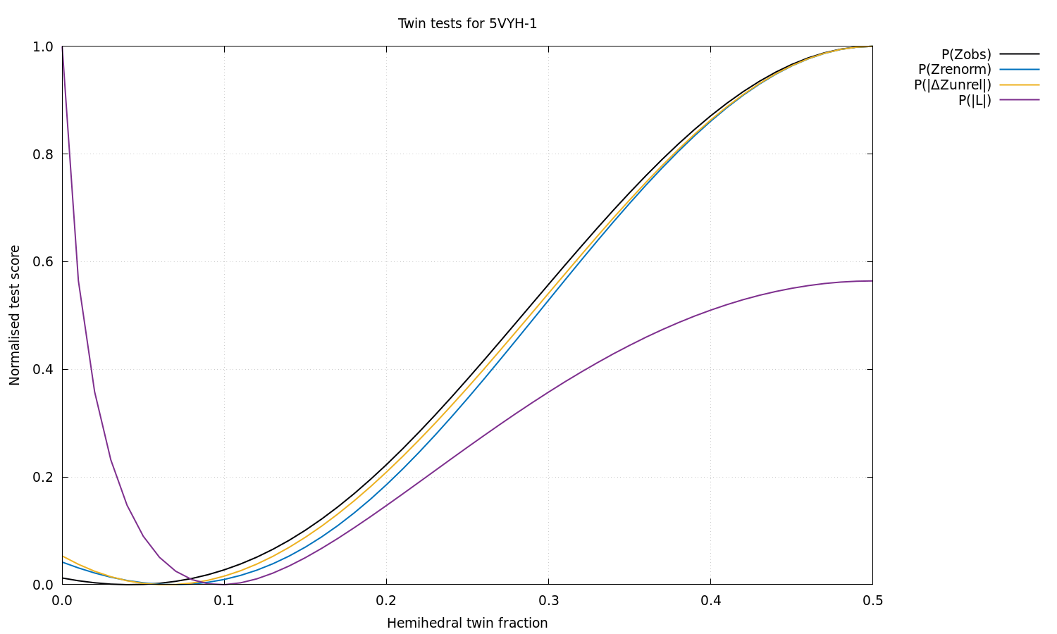
Estimated twin fraction from K-L divergence of observed acentric Z probability (before, after): 0.04 0.07
Estimated twin fraction from K-L divergence of posterior acentric Z probability: 0.07
Estimated twin fraction from K-L divergence of unrelated acentric |delta-Z| probability: 0.06
Padilla & Yeates L test for twinning, acentric moments of |L|:
<|L|> (normal = .500; perfect twin = .375): 0.439
<L^2> (normal = .333; perfect twin = .200): 0.264
Estimated twin fraction from K-L divergence of |L| probability: 0.10
Reference